RMC
|
EXAFS:
Extended X-ray Absorption Fine Structure |
|
Introduction |
XAS (X-ray absorption spectroscopy) is an element specific method to investigate the bond angles, bond lengths and coordination numbers. During the experiment the material under investigation is targeted with monochromatic X-ray beam (produced by synchrotron radiation). Some of the X-ray photons are absorbed by the material, and the rate of the absorption is measured versus the X-ray photon energy.
The X-ray absorption coefficient of a
homogenous material can be given by
![]()
where E is the photon energy and d is the thickness of the sample. Generally, the absorption of X-ray is decreasing with the increasing energy of the X-ray photons, but distinct spikes corresponding to a drastic increase of the absorption can be detected at some energy. These are the absorption edges, and they correspond to the binding energies of the inner-shell electrons (K, L, M..). As each chemical element has specific, well-defined binding energies, it is possible to select an energy range for the X-ray beam sweeping specifically only an absorption edge (and the following) region of a selected element. This way information of the neighbourhood of the atoms of this chosen chemical element can be obtained.
XAS spectrum can be
divided into different parts based on the energy range of the X-ray beam
compared to the absorption edge, but there is no consensus in the literature
neither in the number nor in the limiting energy values of the ranges. A possible division is given here.
1.) Directly before the absorption edge can be
found the pre-edge region, where no ionisation
occurs, only transition to higher, non-completely filled or empty orbits.
2.) In the edge region, where photon energy, E
£ E0+10 eV (E0 is the
ionisation energy) the XANES (X-ray Near Edge Structure) is observable.
3.) NEXAFS (Near-Edge X-ray Absorption Fine Structure) region is between E0+10<E
£ E0+50 eV.
4.) EXAFS region is where E >E0+50 eV.
It has to be noted, that sometimes there is no division
between the XANES and NEXAFS region, and the two acronyms are used as synonyms,
although NEXAFS is usually used in connection with organic molecules and
surfaces. The absorption edge itself sometimes is not considered to be in the
XANES region, and the beginning of this region is set at E > E0+5 eV. Sometimes the division between the XANES-NEXAFS
and EXAFS region is set around 150 eV. From now on the acronym XANES will be
used for the description of the XANES-NEXAFS range. A typical XAS spectrum can
be seen below:
XAS spectrum to show the different
methods depending on the energy range of the X-ray photon. m(E) is the energy dependent absorption
given by E 1, the
energy is given in eV.
|
The structure
of the XAS spectrum |
When the X-ray photon energy reaches the ionisation energy of an inner shell atom, the absorption rapidly increases creating the ascending part of the absorption edge peak. After the maximum the decrease of the absorption is not smooth, but larger and smaller wave crests and troughs are super-positioned on the exponentially decreasing signal. This is the so-called XAFS (X-ray Absorption Fine Structure), which can give statistical information about the local structure around the absorber atoms. The reason for the XAFS is the following. XAFS appear only if there are atoms near the absorbing atom, so in solid and liquid state and in molecular gasses. In case of free atoms as for example noble gasses no XAFS can be observed.
When the X-ray photon with E>E0 is absorbed, its whole energy is transferred to an inner-shell electron, which will jump to unoccupied continuum level with symmetry properties defined by the dipole selection rules. If the configuration interaction is negligible, than the selection rule is Dl=±1. The absorption edges are denoted according to the shell of the ejected core electron (K, LI, LII, LIII). The ejected photoelectron will have kinetic energy E-E0. The outgoing photoelectron wave can be scattered by the neighbouring atoms, and the XAFS is caused by the interference of the outgoing and backscattered electron wave at the position of the absorber atom.
Initial state
|
Final
state |
|
|
K |
2S1/2 |
p |
|
LI |
2S1/2 |
p |
|
LII |
2P1/2 |
d, (s) |
|
LIII |
2P3/2 |
d, (s) |
There is however a difference in the physical phenomenon taking place at low or higher kinetic energy, In the XANES region, where the kinetic energy of the photoelectron is low, multiple scattering of the photoelectron by the neighbouring atoms occurs. This is due to the fact, that the corresponding wave vector of the photoelectron is large enough to be comparable to the inter-atomic distances between the absorber and its neighbours, and the scattering amplitude is large. Due to the multiple-scattering process, XANES probes the 3 and more-body correlations and can give information not just about bond lengths (or inter-atomic distances), but about the bond angles, too.
In the EXAFS region the kinetic energy of the photoelectron
is higher and consequently the wave length and the scattering amplitude is
smaller, so mainly single scattering of the photoelectron by the neighbouring
atoms takes place.
The scattering
amplitude and phase shift caused by the backscatterer depends on of the
neighbour’s type, and the phase and the amplitude of the backscattered wave
depends on the inter-atomic distance between the absorber and the backscatterer
as well.
After the ejection of the photoelectron
the absorber atom will be in an exited state due to the core hole. Relaxation
can occur when an electron occupying a higher energy level jump down into the
core hole. The energy difference between the levels is either emitted as a
fluorescence photon (only rarely occur), or absorbed by an other higher-level
electron, which is emitted from the atom (Auger-electron).
The wave vector of the photoelectron (k)
can be calculated from the X-ray photon energy, E and the ionization
energy, E0 by:
The oscillating absorption coefficient is
normalized by the smooth atomic absorption background, m0
defining the EXAFS signal, c(k):
|
RMC specific
remarks |
Standard EXAFS
It has to be noted, that in RMC c2 is applied for denoting the
difference between the experimental and calculated data, so it should not be
confused with c(k). For fitting EXAFS data in
RMC, the values of k and c(k) has to be given in the EXAFS data file as the input
experimental EXAFS data.
The EXAFS experimental data used in the
fitting is denoted by E(k) and it is
calculated by
after reading
the k and c(k) data from the experimental data file. The weighting
factor n has to be given in the *.dat file, and it is a small
integer usually between 1 and 3. The reason for using this weighting is to
compensate for the amplitude decay, fitting with n=1, 2, 3 results in a
physically more realistic configuration than in case of n=0, kmax
is the largest k value of the data set.
The coefficients, c(r,k) for the
Fourier-transformation of the r-space information to k-space are r,k
dependent, and has to be given in the coefficient file. The coefficients
can be calculated for example by program FEFF, see some information about it here. Care has
to be taken, that the same r-points have to be used during the
coefficient calculation as used in the RMC simulation. Keep in mind, that in
RMC always the middle of the bin is used for the given bin! It is possible to
use only a range of the r-dependent coefficients given in the coefficient file,
this can be specified in the *.dat file. Different ranges can be
specified for the different partials (all the possible atom type pairs of the edge particle type)
for an absorption edge. The minimum and maximum indices of
the r points (columns)
for the partials are given in the *.dat file, in the order rmin1,
rmax1, rmin2 rmax2, ->rminN,
rmaxN, where the indexing refers to the partials contributing to
the given edge. For example for a 3-component system of As, Se, I for the As
edge there are three partials (As-As, As-Se, As-I), for which the r
index data has to follow in RMC order for the partials.
The calculation of EC(k)
data is performed according to the following formula:
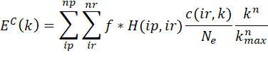
where H(ip,ir) is the value of the ip-th partial
histogram ir-th histogram bin, Ne is the number of the
particles with the absorption edge. The first sum is going through all the
partials containing the particle type producing the absorption edge. The c2 is calculated as
only using constant and
multiplication factor for renormalizations.
Coefficient correction with E0 shift
As there can be some error regarding the coefficient calculation, and the measurement, there is a possibility to try to calculate the E(k) with a somewhat shifted coefficient matrix from version 1.8. A maximum DE0 shift can be chosen, which would mean
|
|
maximum left and right k values, as the relationship between DE0 and k is not linear. To make the calculation quicker,
the shift cannot be any value between![]() . A
symmetric, equidistant 2*N+1 point
grid in the energy space will be created between -DE0 à+DE0,
and the k values for each E-grid points will be calculated according to
. A
symmetric, equidistant 2*N+1 point
grid in the energy space will be created between -DE0 à+DE0,
and the k values for each E-grid points will be calculated according to
where the positive ![]() values correspond to the left (smaller k) part of the k interval and the negative
values correspond to the left (smaller k) part of the k interval and the negative ![]() to the right
part.
to the right
part.
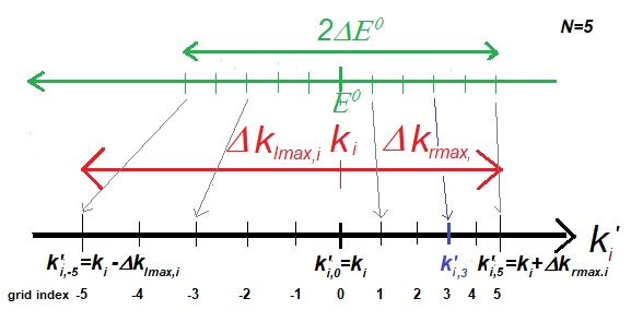
The relationship between DE0 and the equidistant E grid, ![]() , and the
non-equdistant k-grid values in case
of Ngrid=5, and chosen
grid index 3.
, and the
non-equdistant k-grid values in case
of Ngrid=5, and chosen
grid index 3.
The distance of the grid points are different in the left and right
direction, and it is obviously k
dependent. The values of the coefficient matrices for each partial is
calculated with linear interpolation for each grid point, k’i,n, and this coeff(k’i,n,rj)
will be used instead of the original coeff(ki,rj) for the calculation of E(ki). It has to be mentioned
that due to the linear interpolation there will be some data point loss at both
end of the k-range!
At every EXAFS-SHIFTSTEPth generated move, no atomic move is performed
(similarly to the scalable background correction or AXS in case of I(Q) data sets) , but a grid index
between –Ngrid ® +Ngrid is randomly
chosen in case of each EXAFS data set, where E0 shift is performed. The grid index is the same for each
partial of a data set. The EXAFS data E(ki) will be calculated using
the coeff(k’i,n,rj) values. The c2 is calculated, and the move accepted or rejected
the usual way. If the move is rejected, then the old grid index is used for the
subsequent steps, if accepted, then the new one till the following
EXAFS-SHIFTSTEPth generated move. The starting grid index is zero meaning no
shift by default.
This feature is only accessible using the free format input file. In the [
GENERAL ] section optionally the default value of the EXAFS-SHIFTSTEP can be
modeified. For each EXAFS data set in the [ EXP ] section optionally the
DELTAE0_NGRID key word can be given, expecting the maximum E0 shift in eV and the number of grid points in one
direction.
Using this option might indicate that only one segment of the grid points
is used. In a following simulation therefore we might one to constrain the
number of used grid points to this segment, and even like to continue the
simulation with a grid point with non-zero grid index, which means using an
asymmetrical grid. To make this possible, an other keyword, E0GRID-FROM_TO_START
was introduced expecting 2 parameters for the first and last grid point to use
and a third, optional value for the grid index to start the simulation with. If
this keyword is given for a data set, then DELTAE0_NGRID should be also given for it, as this
latter specifies the grid.
The shifted coefficient matrices are only calculated for the used grid
points. The data points loss is determined based on the whole symmetrical grid
given by DELTAE0_NGRID.
For example if the following lines are present for a EXAFS set:
DELTAE0_NGRID = 2 5
E0GRID-FROM_TO_START = -3 1 -2
then only the blue range given in the figure below will be used representing E0 shift values 1.2 à-0.4
eV, starting with 0.8 eV shift.
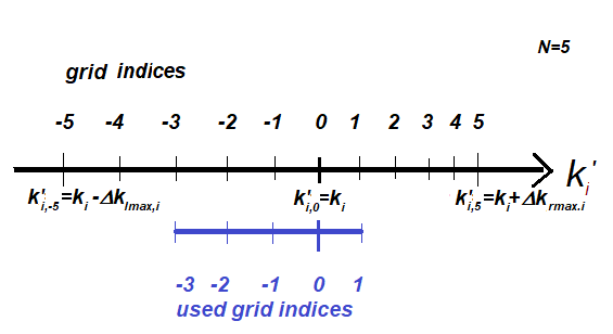
The usage of the asymmetrical E0 shift grid, where the
original grid has 5 shifted grid points in one direction, and only the -3 à 1
range is used.
|
Links |
There are plenty of more detailed
descriptions of EXAFS in the Internet, for example:
Last modified 04/03/2023) by Orsolya Gereben
(comments welcome!)