RMC
|
RMC++ in short |
|
Description
of the algorithm |
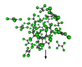
The spatial distribution of
atoms and molecules in a disordered material is described by the so-called
partial pair correlation functions.
|
|
|
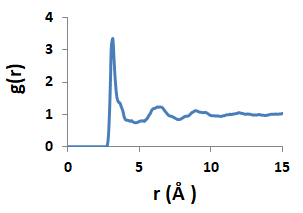
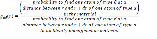
Definition of the partial pair correlation
functions
The structure can be probed
by the diffraction (elastic scattering) of waves (neutrons or X-ray electron
diffraction) of adequate wavelength . The partial
structure factors are obtained by sine-Fourier transform from the partial pair
correlation functions:
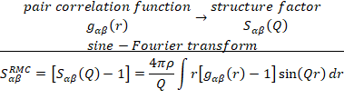
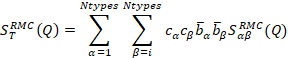
and the diffracted intensity is a linear combination
of the partial structure factors Sab(Q), where Q is the scattering vector, weighted by the concentrations c
and scattering lengths b:
It
has to be noted, that in RMC the partial and total structure factors defined as
above that they tend to zero at large Q values, and the experimental data is
interpreted as such.
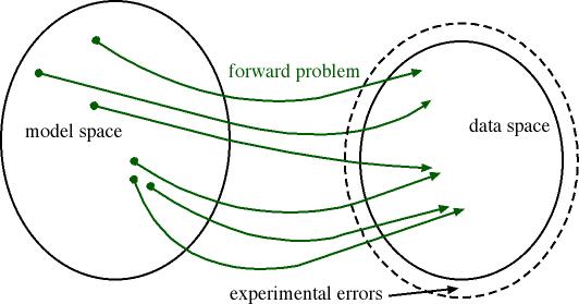
Direct inversion of this inverse problem needs several
measurements with isotopic substitution to disentangle the different partials.
Furthermore, it is plagued with the usual problems of instability, over- and
under-determination, and the Fourier ripples due to truncated Q-range.
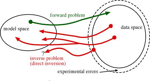
Forward and inverse problems
One alternative solution to
direct inversion, is to explore the parameter space
and solve the direct problem as often as required.
Repeated computation of the forward problem
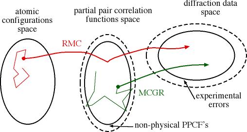
In MCGR [Monte
Carlo modelling of G(r)], the parameter space consists in the
discretised pair correlation functions. This technique allows to model partials
while avoiding some of the usual pitfalls of direct inversion (still, it does
not guarantee that the partials are physically sound).
Reverse Monte Carlo (RMC) goes one step further and considers the positions
of a set of N atoms (the configuration) as the parameter space, i.e.
it will derive a set of coordinates of the N atoms of the configuration that is
in agreement with the data.
MCGR vs. RMC
Systematic or exhaustive exploration
of the parameter space is ruled out by its mere dimension, and therefore a more
efficient way of sampling is needed in order to converge towards one
solution.
Both MCGR and RMC are based on the Metropolis algorithm, i.e. the
parameter space is explored by a `guided' random-walk. In short, the acceptance
of generated random moves in the parameter space is defined by the agreement of
the corresponding calculated data with the experimental data.
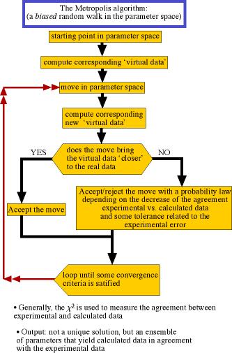
Flowchart of the metropolis algorithm
In `standard' RMC++ (as in
the existing RMCA) the random move in the parameter space consists in the
displacement of one atom of the configuration. The atom
moved, as well as the amplitude and the direction of the move is defined
randomly (within some predefined range).
One essential additional component in RMC is the introduction of constraints.
The Metropolis algorithm indeed produces solutions with the largest amount of
disorder, for a given set of constraints (including the c2). Constraints can be introduced at 2 stages in the
algorithm:
- at the definition of the move i.e.
reject moves that bring atoms to close to one another (distances of
closest approach).
- at the definition of the c2, by adding terms corresponding
to coordination constraints or potential.
Individual
molecules can also be mimicked by imposing a distance range between defined
atoms in the configuration (the so-called fixed neighbour constraints - FNC
-).
The flowchart of the `standard' RMC algorithm appears below:
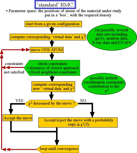
Flowchart of the RMC algorithm
For more details, look at the
references.
|
Description of the potential using algorithm
|
In 2010 the algorithm was
amended with the usage of non-bonded and bonded potentials. Bonded potentials are
an new way to keep molecules together as an
alternative to FNC. Non-bonded potential can be used together with it, or it
can be useful for atomic systems as well. The potential-using RMC simulations
are closely linked with molecular dynamics (MD) simulations, as the potentials
and the parameters to use usually come from force fields developed for MD, see
some papers about it on the references page.
The algorithm will not be
discussed here in details, only the flowcharts are given here:
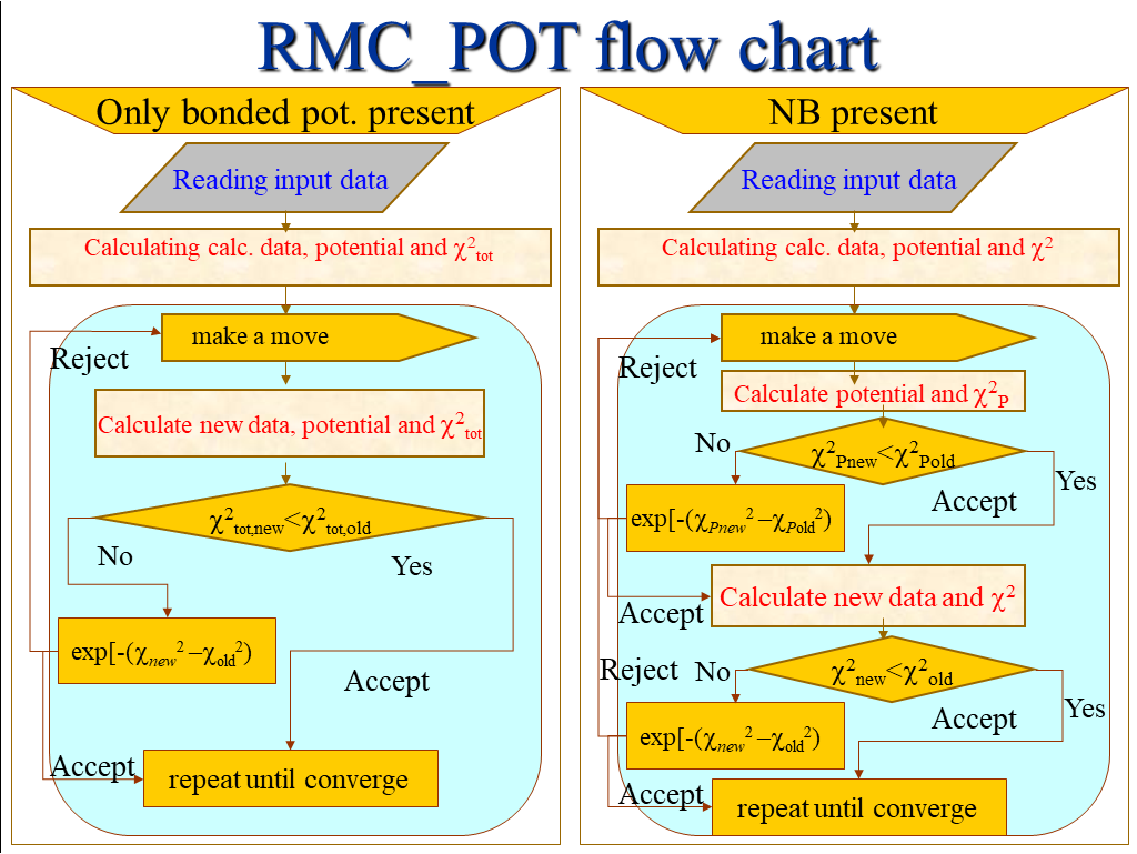
Left: Flowchart of
the only-bonded potential-using RMC algorithm (where the potential-related c2 is
added to the normal c2. Right non-bonded potential also used, a separate,
potential related cP2 is
evaluated first, and if it accepted, then follows the c2 test
of the data sets.
|
RMC implementations |
The
different RMC implementations can be found on the development
history page.
The
earlier versions of RMC++
should look very familiar to RMCA users, since it uses the same input
and similar output format. Later on due to the increasing number of new
features the fixed format input file *.dat was changed to free format to be able to
accommodate the parameter input for the new features, although for the old
features the old, fixed format still can be used.
Look at the examples to see what can be done with RMC.
Look at the manual for details concerning input and
output.
Last modified 04/03/2023) by Orsolya Gereben
(comments welcome!)