RMC
|
RMC++ topics |
This page describes specific topics relevant to the use of the RMC
algorithm in general, and of RMC++ in particular.
The problems discussed below
include:
·
the
requirements on r-space discretization due to the Q-range of the data
·
the
definition of the configuration size
·
the
normalisation of the histograms
·
Uncertainty relation for g(r) partials
Link to topics discussed separately
are the following:
·
quadratic background correction
The newest features are not discussed
here, see the manual:
·
local
invariance
·
non-periodic
boundary condition simulations
·
X-ray
intensity fitting
·
advanced
geometric constraints: Second Neighbour Constraint, Common Neighbour
Constraint, Bond Valence Constraint
·
ANN
potential (see also the AENET website)
The first thing to do in a
RMC run is to define the configuration that will be simulated.
The choice of the configuration size, the Q-range of the data and
the histogram bin width are linked by mathematical requirements
intrinsic to the method, by finite computer time, and by what kind of information
is expected from the RMC simulation (this latter being actually the most
important).
|
The
histograms bin width |
- The bin width dr of
the histograms interval must be small enough to allow the approximation of
the sine-Fourier transform for the data points up to the highest Q-value.
This requirement reads:
![]()
- The bin width dr
defines the resolution of the final g(r) partials. But logically,
fine details in the g(r)'s can only be constrained by high Q-values
(i.e. the relevance on the high resolution details in the g(r)
should be estimated from the Q-range)
- What is more, the finer the r-bins, the fewer
distance in the bins, and therefore, the greater the
statistical uncertainty on the derived g(r) values. So for smaller
bins only makes sense for large system.
- The usual bin size is 0.1 Å for a system
containing <10000 particles. If there is more than one component, than
the histogram counts will be divided among the partial histograms, so the
statistic will be worse than for a mono-atomic system.
In short, the
bin width dr should be chosen as large as
possible, taking into account the maximum Q-values in the data and the
desired degree of detail in the g(r) partials.
|
The
configuration size |
- The configuration size (i.e. the largest
distance binned in the histograms) must be greater than the minimal range
after which there is complete disorder (i.e. positions of atoms are
not correlated and the partial pair correlation functions take the value
1).
This is a mathematical requirement for the approximation of the sine-Fourier transform - The number of atoms must be as large as possible for
the sake of statistical accuracy. The density being fixed, that means that
the larger the configuration the better. From a `hand waving' argument, it can be seen that there is
a relation between the statistical uncertainties on the derived g(r)
values at small r-range, the bin width dr,
and the total number of atoms N which reads:
![]()
Note
that at the moment, there is no tool for assessing the uncertainties on RMC
results.
- On the other hand, the number of distances
calculated for each move grows as N, and this is the most
time-consuming part of the algorithm.
In short, the
configuration size (and the optional xmax value
extending the histogram range beyond the half-size of the cubic box in RMC++)
must be chosen as large as possible, for the computing time available.
Note that in general it is not the long range order that fixes the
configuration size, but rather the statistical uncertainty due to small bin
counts at small distances. In other words, the configuration size is dictated
by the r resolution that one wants rather than from the long range order
of the material.
|
The
normalisation of the histograms |
In RMC, the g(r) partials are
estimated by counting and binning distances between atoms in the configuration.
This operation requires the renormalization of the histograms defined by
![]()
where i is the bin index, r
the corresponding radius (distance), ρ the number density, dr the histogram bin width and S a surface factor. If the
sphere of radius r is contained in the configuration box, the the factor S is just the surface of this sphere.
In RMCA only distances in this case are considered: if L is the (half) size of the configuration box, histograms (and partials) are
computed up to L. In other words, for a central atom, only neighbours up to a
distance L are used for the computation of the histogram. This means that (4/3
πL³)/(8 πL³)=52.3 % of all
available (and computed) distances are effectively used for the g(r)
computation.
In RMC++, this range can be extended by using the appropriate surface factor.
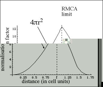
The maximum distance range is √3 L, and there is an analytical formula
for S up to √2 L (see RMC++ manual).
This allows using a smaller box with systems with long range order. But as
noted above, the limiting factor for the configuration size is usually the
number of centres.
If non-periodic boundary condition is used (see the RMC_POT user
guide), and the
system is simulated as a spherical particle in the middle of the simulation
box, then the volume elements has to be normalized differently, which can be
found in the user
guide, or here.
|
Uncertainty
relation for g(r) partials (handwaving argument) |
For
disordered materials, one focuses on "local" order, i.e. how
neighbouring atoms are arranged.
In RMC, the g(r) partials are estimated via the histograms of distances. The
number of distances in the spherical shell [r, r+dr] grows as r squared, but
'locally' (i.e. at very short range) it is proportional to the number of
centers (i.e. number of atoms N).
This number of 'local' distances is shared between the histogram bins, whose
number is proportional to 1/dr.
The average number of local distances per bin is therefore proportional to N
dr, and the uncertainty on this number (standard
deviation) is therefore proportional to (N dr)^(1/2).
The partial g(r) is obtained by normalising the histograms, and the normalising
factor is proportional to dr. Consequently,the derived (absolute) uncertainty (standard
deviation) on the g(r) partial reads
![]()
However, for the relative statistical uncertainty on g(r) one has:
![]()
which indicates that for maximum precision, the number
of atoms in the configurations must be chosen as large as possible, and that
any gain in r-resolution is paid by a loss in the g(r) precision.
Last modified 04/03/2023) by Orsolya Gereben
(comments welcome!)